View the Project on GitHub MissouriMRDT/RoveSoSimulator
- Home
- Getting Started
- Linux Setup Help
- Documentation
- Diversion
- Importing Rover
- Lidar Point Cloud Generation System
Technical Documentation: Lidar Point Cloud Generation System
Project Goal: To develop a robust, high-performance tool within Unreal Engine capable of generating large-scale, georeferenced lidar point clouds. The primary objective is to emulate the format and structure of real-world USGS lidar datasets to facilitate high-fidelity “Sim-to-Real” testing for robotics applications.
Chapter 1: Architectural Overview and Key Design Decisions
The core challenge of this project was to scan a massive (4km x 4km) virtual landscape and export billions of data points without running out of memory or freezing the editor for an unacceptable amount of time. This required several key architectural decisions.
1.1: Core Technology: Grid-Based Ray Tracing in C++ To achieve the highest fidelity, we opted for a Grid-Based Ray Tracing method. This technique simulates an aerial lidar scanner by casting a dense grid of parallel rays from the sky downwards. The primary logic was implemented in C++ for three critical reasons:
- Performance: The sheer number of calculations (billions of ray casts) is far too slow to be handled by Blueprints. C++ provides the necessary speed.
- Precision: Geospatial coordinates require
doubleprecision to avoid significant errors over large distances. C++ handlesdoublesnatively, whereas Blueprints primarily usefloats. - Memory Management: C++ provides the low-level control needed to manage memory efficiently, which is crucial for the chunking system.
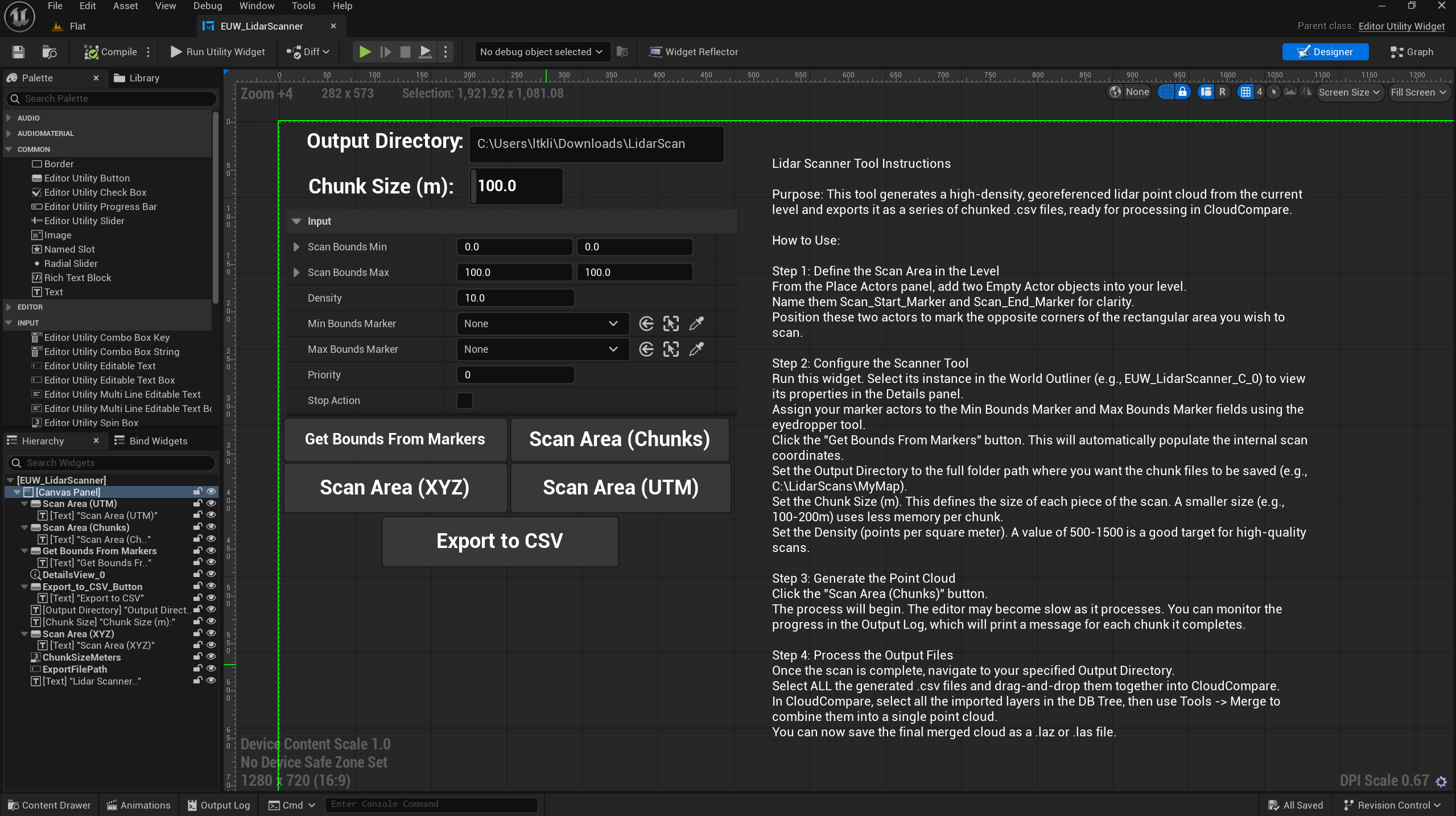
1.2: User Interface: The Editor Utility Widget
While the core logic is C++, the user interface is a Blueprint Editor Utility Widget (EUW_LidarScanner). This provides a friendly, visual front-end that allows any team member (not just programmers) to use the tool. The Blueprint’s role is simply to gather user inputs and pass them to the C++ backend.
1.3: The Memory Challenge: A Chunking (Tiling) System Our initial prototype attempted to generate and store all points in a single large array in memory. This approach failed due to extreme memory consumption (roughly 1GB of RAM per million points), making it impossible to scan the full map.
- The Solution: We re-architected the system to use chunking. The C++ “manager” function divides the total scan area into a grid of smaller, manageable chunks (e.g., 200m x 200m). A “worker” function then processes only one chunk at a time, writing its results directly to a unique file on the disk before its memory is released. This ensures that memory usage remains low and constant, regardless of the total scan size.
1.4: The Performance Challenge: Parallel Processing The chunking system solved the memory issue, but processing hundreds of chunks sequentially was still time-consuming.
- The Solution: We identified that the processing of each chunk is completely independent. This “embarrassingly parallel” problem was a perfect candidate for multithreading. We implemented Unreal Engine’s
ParallelFortask system, which distributes the processing of all chunks across all available CPU cores. This change resulted in a massive, near-linear speedup, reducing scan times from hours to minutes.
1.5: The Export Format: Intermediate CSV for CloudCompare
Directly exporting to the complex, binary .laz format would require integrating a large, third-party C++ library, a significant and often fragile engineering task.
- The Solution: We opted to export each chunk to a simple, human-readable Comma-Separated Values (
.csv) text file. This has several advantages:- Simplicity: Writing a text file requires only built-in Unreal C++ functions.
- Debuggability: The output can be opened in any text editor or spreadsheet program to instantly verify the data.
- Leverages Best-in-Class Tools: The industry-standard software CloudCompare is exceptionally good at importing, merging, and converting point cloud data. Our workflow offloads the final, complex file conversion to this dedicated tool, guaranteeing a 100% compliant
.lazfile.
Chapter 2: The C++ Implementation Details
The core of the system resides in the LidarScannerLibrary C++ class, which contains two primary functions.
2.1: The “Manager” Function: ScanWorldInChunks()
This is the high-level function called by the Blueprint UI. Its responsibilities are:
- Verify that a
GeoReferencingSystemactor exists in the world. - Export a
_CRS_Info.txtmetadata file containing the UTM zone (Projected CRS) for the dataset. - Calculate the grid of chunks based on the total scan area and the user-defined chunk size.
- Prepare a list (
TArray) of “task” structs, where each task contains the specific bounds and output filename for one chunk. - Dispatch all tasks to the
ParallelForsystem to be executed across multiple CPU threads.
2.2: The “Worker” Function: ScanAndExportChunkToCSV()
This function is executed by each thread from the ParallelFor loop. It performs the actual work on a single chunk:
- Creates a temporary array to hold the points for only its assigned chunk.
- Performs the nested loop for the ray-tracing grid.
- For each successful ray hit:
- It gets the hit location in Unreal coordinates.
- It calls the
GeoReferencingSystem’sEngineToProjectedfunction to convert the location toFProjectedCoordinates(Easting, Northing, Altitude). - It performs classification logic by checking the tags of the hit actor.
- It adds the final, complete
FLidarPointstruct to its temporary array.
- Once the scan for its chunk is complete, it formats the data into a series of strings.
- It writes all the formatted strings to its assigned
.csvfile on disk usingFFileHelper::SaveStringArrayToFile.
Chapter 3: The End-User Workflow (How to Use the Tool)
This guide outlines the complete process for a user to generate a point cloud.
Step 3.1: Scene Preparation
- Place GeoReferencing Actor: Ensure a properly configured
GeoReferencingSystemactor is present in the level. The Projected CRS and Origin Location must be set correctly. - Place Marker Actors: Add two
Empty Actorobjects to the level. Position them at opposite corners of the desired total scan area.
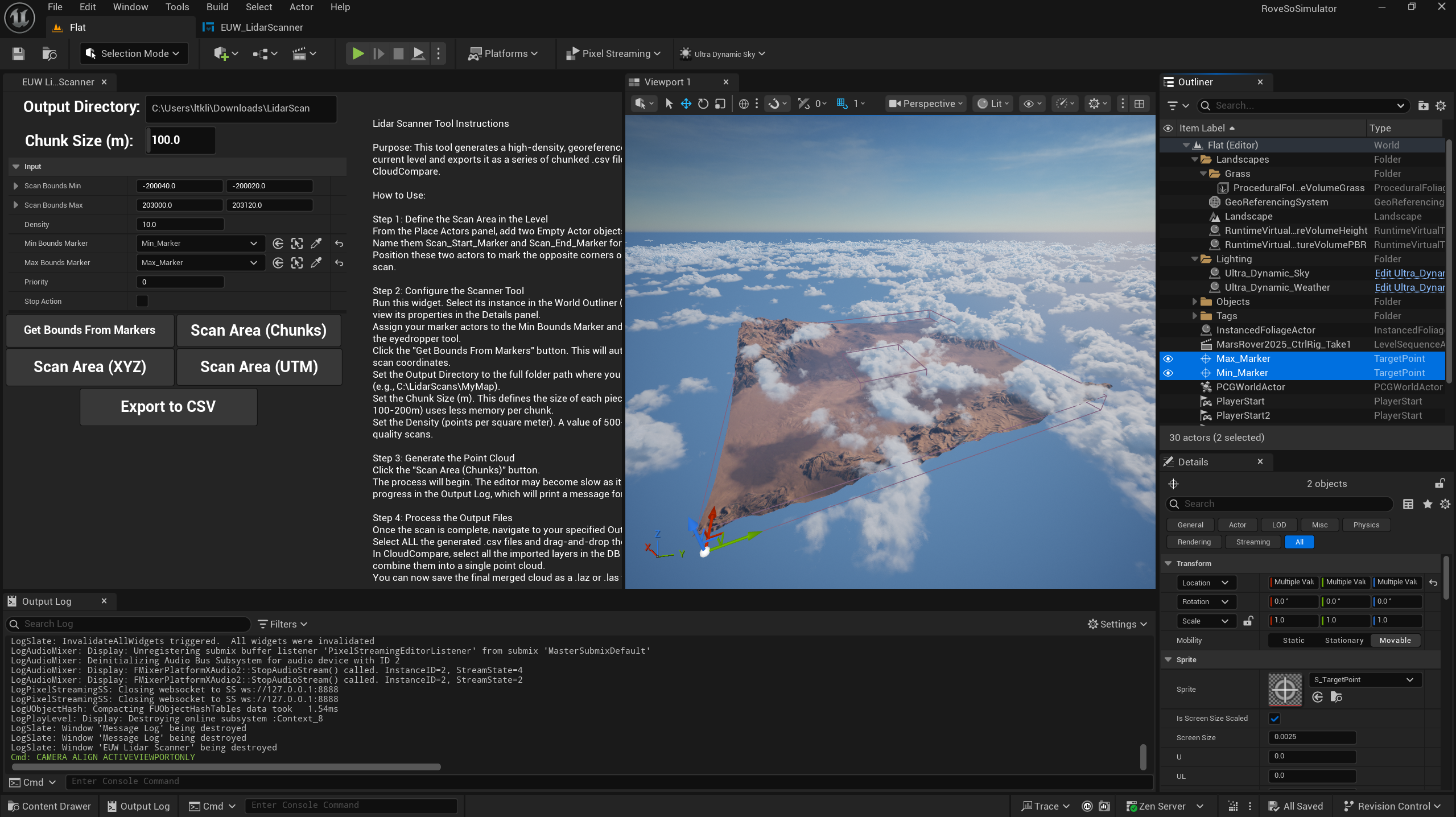
Step 3.2: Configure and Run the Scanner Tool
- Launch the Widget: In the Content Browser, right-click the
EUW_LidarScannerasset and selectRun Editor Utility Widget. - Select the Widget Instance: In the World Outliner, click on the running widget instance to make its properties appear in the Details panel.
- Assign Markers: Use the eyedropper tools to assign your two marker actors to the
Min Bounds MarkerandMax Bounds Markerfields. - Get Bounds: Click the “Get Bounds From Markers” button.
- Set Parameters:
- Output Directory: Provide the full path to a folder where the output files will be saved.
- Chunk Size (m): A value of
100to500is recommended. Smaller chunks use less RAM. - Density: Set the desired points per square meter.
- Execute Scan: Click the “Scan Area (Chunks)” button. The process will run in the background. Progress can be monitored via the
Output Log.
Step 3.3: Final Processing in CloudCompare
- Import: Once the scan is complete, open the output directory. Select all the generated
.csvfiles and drag them simultaneously into the CloudCompare window. - Merge: In CloudCompare’s
DB Treeview, select all the newly imported layers. Navigate to Tools -> Merge. This will combine all chunks into a single entity. - Export: Select the final merged point cloud. Go to File -> Save. In the save dialog, choose the desired file type (
.lazfor compressed,.lasfor uncompressed) and save the final output file. The metadata from the_CRS_Info.txtfile can be used to set the coordinate system information in the target application.